Two Boulders on Mt. Blue Sky 🗻

Let’s see the math in action! I applied this model to a case study by comparing two climbs on Mt. Blue Sky, Colorado: “Clear Blue Skies” and “No More Greener Grasses.” There is much debate about whether each climb is “V11” or “V12.” These two climbs were chosen because of their proximity which somewhat controls for the effects of environmental factors; on the other hand weather in the alpine is highly variable, so perhaps not. They sit only feet from each other on the same piece of rock. Also, both climbs see many repeats every year, providing the necessary quantity of data. Studying these problems isolates significant factors that impact climbers’ reported grades.

While the climbs are adjacent to each other on the Dali wall, they pose different challenges to a climber. First, “Clear Blue Skies” (CBS) sits in the middle of the wall with brutally small holds that are slippery to the touch. On the right side of the wall is “No More Greener Grasses” (NMGG). After discussions with many expert climbers, it is well understood that the difficulty of CBS mostly derives itself from making relatively small but powerful moves between these small holds. NMGG is a similar number of moves, but it covers much more distance. The holds are larger, and the wall is steeper. Currently, both are considered to be graded around “V11” or “V12,” but their history is rich and people’s opinions surrounding the relative difficulty of each climb is fraught with controversy.

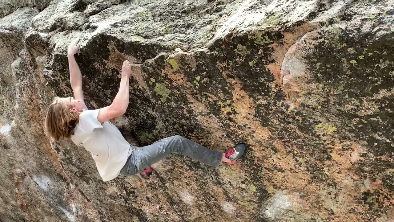
Elite climber Jess Walker climbing Clear Blue Skies

At the time of writing, it is more common for ascensionists to grade CBS as “V11” and NMGG as “V12.” From anecdotal reports, both take a similar amount of effort and time to complete. This indicates the climbs are comparable. It appears that CBS suits a narrower range of body morphologies and competencies, and NMGG is more amicable to a broader range of morphologies and competencies. The models described are applied to analyze these two climbs.

Obtaining the Data

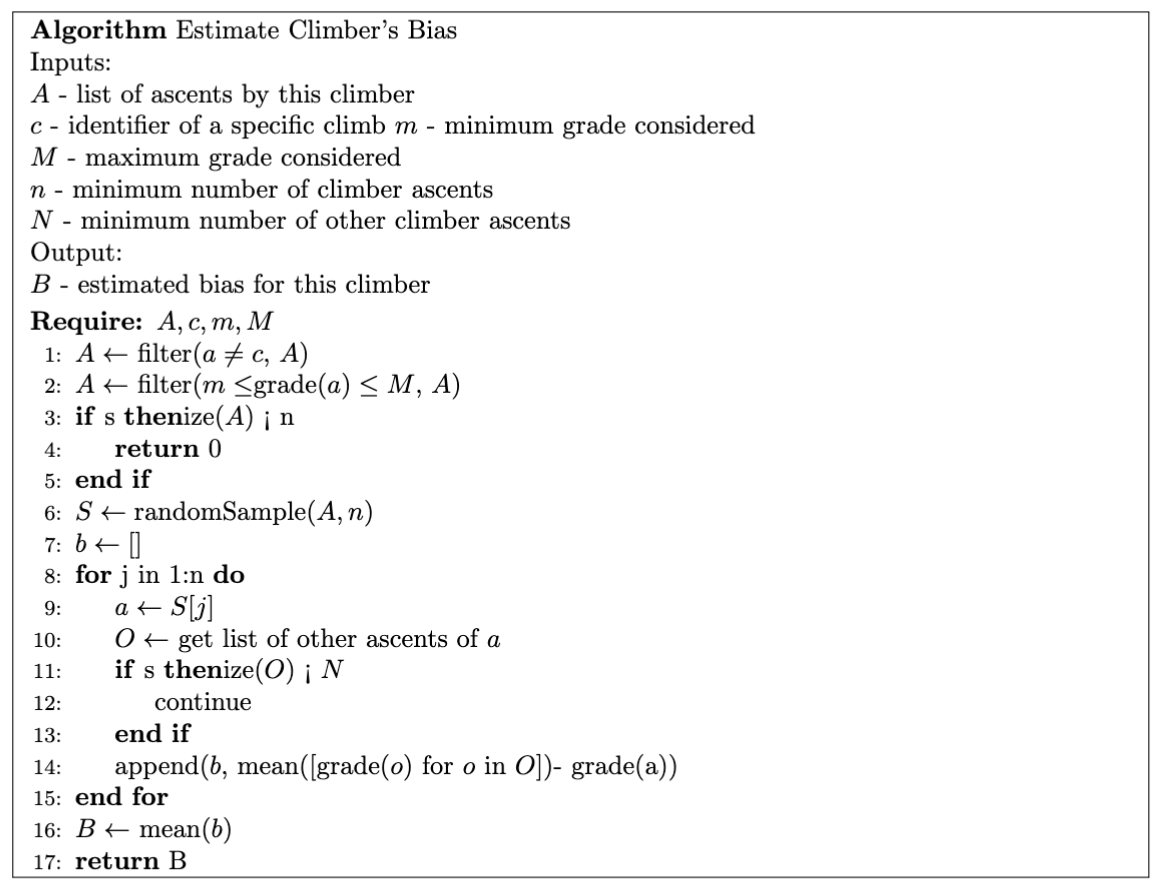
A considerable amount of effort 👨‍💻 was spent obtaining access to the world’s largest collection of reported climbing grades on 8a.nu in such a way as to leverage the data. 8a has been used as the primary logging platform for elite and casual climbers for the last two decades. The database gives a unique opportunity to use statistical and computational tools. I collected all logged ascents of the climbs until the spring of 2023 and then estimated the bias for each climber who has done the climb with the algorithm I mentioned earlier. I subtracted the estimated biases from the reported grades to obtain samples of the experienced difficulty. This involved going through the publicly available web interface and isolating the data for each ascent. Programmatically, each ascent is then represented as a collection of the following fields:

• Ascensionist’s Name
• Reported Grade: reported as an integer
• Hard/Soft Label: this specifies if the ascensionist believes the grade is difficult or easy for the grade respectively
• Algorithm Grade: The integer reported grade is digested into the algorithm as that integer plus 0.5 to place it directly between the grade above and below. For instance, a “V11” would be interpreted as 11.5. The hard and soft identifiers modify the grade by 0.25, so a “hard V11” would be considered 11.75. A “soft V11” would be 11.25.
• Other qualitative descriptors: These are not incorporated into the analysis, but may be useful in follow on work. For instance, this data could help incorporate physical conditions or personal aptitudes when considering conditional distributions.

Estimating Grade Distributions

We assume the form of each distribution, and then this becomes a parameter estimation problem. This was done through third party software from SciPy and scikit-learn. Both are python packages widely used for machine learning and statistics. The Normal and Gamma distribution’s parameters are estimated using maximum likelihood estimation (MLE). For the Gaussian Mixtures the parameters are estimated via expectation maximization. It is worth noting that parameter estimation generally is a non-convex nonlinear optimization problem and thus there are few guarantees that we estimate the parameters well. In practice, parameter estimation is necessary, and thus we must try. The techniques used here are standard and used in the sciences widely.

Assessing the Distributions

You might ask:

“How good of a job am I doing?”

I want to know that as well. Good for us, mathematicians have developed ways to evaluate how well a distribution matches a sample.

The first thing to do is a qualitative analysis: look at the histogram of the debiased grades with a fit distribution superimposed. This can give a valuable qualitative picture of if the fit distribution “looks right”.

You should feel unsatisfied with that step, and should ask, “How should the fit distribution be evaluated quantitatively?” There are many metrics one could consider, but one with a particularly interesting interpretation is the Kullback-Leibler divergence (KL divergence) defined below. Mathematically, this divergence is rich in meaning, but in this application, it can be interpreted as the “expected surprise” by choosing the fit distribution rather than some true distribution. The KL divergence measures how well the choice of model describes the true behavior of the data.

$D_{KL}(p||q)={\int }_{-\infty }^{\infty }p(x)\log \left(\frac{p(x)}{q(x)}\right)dx$

where $p$ is the probability density function PDF of the fit model, and $q$ is the PDF of the true distribution.

If the KL divergence is small, the fit distribution is, in some sense, equivalent to the true distribution. If the KL divergence is large, the fit distribution does not represent the true distribution. Comparing KL divergences between models can help determine which model better fits the data, i.e. the model with the smaller KL divergence in general is better.

An important caveat to note is that the KL divergence cannot be computed exactly for any of the candidate models because the exact distribution is not known. Instead, the KL divergence is estimated by using the cumulative distribution function (CDF) of the fit distribution and the empirical CDF of the data, see this paper for more details. This is shown to asymptotically converge to the true KL divergence, so as the size of the data set increases, so does the accuracy of the estimate.

${\hat{D}}_{KL}(p||f)=\frac{1}{J}{\sum }_{n=2}^N\log (\frac{\delta P_n}{\delta Q_n})$ where $\delta P_n$ is the difference in the fit distribution’s CDF from the ordered data $n-1$ to $n$, and $\delta Q_n$ is the difference in the empirical CDF from the ordered data $n-1$ to $n$.

Clear Blue Skies

For all of the available debiased CBS grades, I fit the Uniform, Gamma and Normal distributions to the data, as well as a Gaussian Mixture, and KDE. We see that the Gaussian Mixture or KDE performs best.

No More Greener Grasses

For all of the available debiased NMGG grades, I fit the Uniform, Gamma and Normal distributions to the data, as well as a Gaussian Mixture, and KDE. We see that the Gaussian Mixture or KDE performs best.

The KL divergence varies depending on which distribution is used. It may be tempting to blindly select the Gaussian Mixture for both climbs because it does minimize the KL divergences. However, qualitatively CBS appears to have two modes (peaks) while NMGG visually has one mode with a single outlier. Thus, the Gaussian Mixture and the KDE could be overfitting the data in the case of NMGG and likely selecting the Gamma or Normal distribution is more prudent.

Todo

Another way to investigate how well our fit distributions match the data is the Kolmorgorov-Smirnov Test(KS Test). The KS Test computes the probability that the data came from a specified distribution. In our case this is almost looking at the process of estimation in reverse. We are asking if the samples of debiased grades could have come from the fit distributions.

Convergence to a Distribution

Oftentimes, climbers will say that the grade has come to a consensus. This means that while there may have been disagreement on the grade during early ascents, at some point the community comes to an agreement that the climb is a particular grade. Culturally, the consensus grade is valued. Sometimes, this consensus is a calculated average. Many websites collect logbooks of ascents and corresponding grades. Two of the most relevant are 8a.nu and 27crags.com. Still, it is often decided by a de facto authority figure like a guidebook author who may or may not have a strong ability to assess difficulty.

Mathematically, this hypothesis can be tested to see what grades actually converge to. If in fact a climbing grade converges to a single number as the number of ascents increases, the fit distribution eventually becomes more and more sharply peaked around a specific number. This is called a Dirac function. If on the other hand the grade converges to a distribution then there is proof that a grade is not a single number, but instead a random variable.

The fit distributions form a sequence $\{F_{d_n}{\}}_{n=1}^N$, and if the distribution is converging to a single number then this would be shown by the limit converging ${\lim }_{n\to \infty }{F}_{d_n}=C$ where $C$ is a constant. Algorithmically, convergence can be met when consecutive elements in the sequence get close to each other $D_{KL}(F_{d_n}-d_{n-1})\le ϵ$. where $ϵ$ is a small number corresponding to an error tolerance. In practice, this means that after a certain number of ascents $n^{\ast }$ if the $D_{KL}$ is small enough, then $F_{d_{n^{\ast }}}$ can be used as a proxy to the data. In essence, now the distribution of the grade is known, and it is the same as $F_{d_{n^{\ast }}}$.

In the histograms in the section above, both CBS and NMGG have not converged to a single grade as seen clearly in the data. But what about the fit distributions? Below are plots of how the KDE changes as more ascents occur over time. The ascents were ordered in time, and then a distribution was fit to a subset of the data, starting with the first ten ascents, then adding one ascent and then another and so on. The KL divergence between fit distributions is computed to see if the sequence is in fact converging. For those who don’t commonly see logarithms, recall as $\log (D_{KL})$ approaches $-\infty$, $D_{KL}$ approaches 0.

Clear Blue Skies

On the left is a surface of fit distributions, and on the right is the pairwise KL divergence between the adjacent fit distributions.

No More Greener Grasses

On the left is a surface of fit distributions, and on the right is the pairwise KL divergence between the adjacent fit distributions.

A Gaussian Mixture model was selected for CBS, and a Normal distribution was used for NMGG. Setting $ϵ=10^{-8}$, both sequences can be considered to have converged. This demonstrates that the climbs are in fact generating a grade that is random rather than a fixed number.

How Hard are These Two Climbs?

What do you gain from using this model over the conventional consensus or personal integer grade? For one, these fit models can be interpreted into actionable information. If one were to integrate under the curve from 0 to 11.75 for the Gaussian Mixture fit to the ascents of CBS, they would get $\approx 54\%$. This represents the probability that someone would experience a “hard V11” or less. One could then use this information to prepare themselves for the likelihood that they might experience a “V11” but there is almost an equal probability that they will experience “V12”. Using the same process for the fit Gamma distribution for NMGG, one can only expect a $\approx 2\%$ chance that they will experience a “hard V11” or less.

Clear Blue Skies

We see that the probability that a person would experience “V11” on CBS, is actually quite high. This means that without knowing anything about a particular climber, we can say that in general one can probably expect to feel like CBS is a hard “V11” or easier.

No More Greener Grasses

In contrast, the data shows that most people expierence NMGG at a grade of “V12” or harder.

To me this is slightly surprising! I definitely think that CBS feels more challenging. This could be because on my specific body morphology, the conditions when I attempted the climb, my lack of ability to assess difficulty accurately, or my bias. Another aspect to consider is that this data analysis does not account for the tendency of the whole community to report a grade that others have taken. The model could be updated model by having the bias depend on the current grade distribution. I think the data may be skewed due to this effect. Thus, as with everything take this analysis with a grain of salt.

Regardless, the exercise of diving deep and seeing what story the available data tells was insightful (and I had a good time). I have done more work with this statistical framework that hopefully will improve the analysis, but polished write ups are not ready to share at the moment. Even if there are obvious limitations in this particular approach, I hope introducing others to think about grades in this way will spark good conversations. I would encourage the reader to see these other qualitative takeaways as well.

Acknowledgements

This is not just my brain child 🧠👶. Thoughtful conversations, edits and ideas were contributed by: Will Anglin, Carlos Tzacz, Dr. Dale Jennings, Dr. Jem Corcoran , Dr. Stephen Becker, Paige Witter, Sam Struthers, Ethan Rummel, and Jeremy Abraham